Finding absolute maximums and minimums of a 2-variable function on a closed region

Tonight, on the World's Most Extreme Values. One 2-variable function. One closed region. One shot at glory. Don't miss it!

...sorry, had to get that out of my system. The problem we're going to look at today goes like this:

Find the absolute minimum(s) and maximum(s) of the function \(f(x,y)=xe^y-x^2-e^y\) on the rectangle with vertices \((0,0)\), \((0,1)\), \((2,0)\), and \((2,1)\).

Ok, we've seen extreme value (i.e., maximum and minimum) problems like this in Calculus 1. If you don't remember the gist of this, please go back and check your notes/textbook first. Just to review, the basic idea is that we find the derivative of a function, set it equal to zero, and solve the resulting equation. Together with the points where the the function is non-differentiable, these solutions give us a set of critical points where the function might have a maximum, minimum, or inflection point.

Our example has two new issues we must confront. First of all, we have a function of two variables, so what does it mean to "set the derivative equal to zero?" Secondly, we have to find the absolute maximums and minimums on a closed region.

Well, the first issue is fairly straightforward. The analogous concept of the first derivative in multi-variable calculus is the gradient, i.e. \(\bigtriangledown f\). But the gradient is a vector, not a scalar - how do we "set it equal to zero"? Well, it turns out that we just set each component (the \(i\) and \(j\) components) equal to zero, and solve the resulting system of equations. Instead of getting solutions that are just \(x\)-values (that we plug in to the function to find \(y\)), we'll get solutions that are pairs of \((x, y)\) values that we'll plug in to find \(z\). As you can see, everything tends to "move up" by a dimension. Since we're moving from planar 2-D functions (curves) to 3-D functions (surfaces), our critical points should be 3-D points as well - they should look like \((x, y, z)\).

The second issue is a little more complicated. If you'll recall from Calc 1, to find absolute extreme values on a closed interval, we needed to check the value of the function at the endpoints of the interval. Then, we needed to compare that value to the value of the function at any critical points inside the interval. Why, you ask?

Well, once we confine ourselves to a closed interval, there is no longer any guarantee that the curve will be flat (or non-differentiable) at the maximum or minimum value. It could very well continue to increase or decrease once we leave the interval. In that case, the point right on the border might be the maximum or minimum of the curve.

For example, consider the problem of finding the highest elevation on Earth - well, that's going to be Mount Everest. But now consider the problem of finding the highest elevation in Kansas - a closed, bounded region. Kansas is very flat, but as you travel east to west, it slowly rises up towards the Rocky Mountains. The highest point in Kansas therefore turns out to be right on the border with Colorado at Mount Sunflower - which isn't really a mountain at all! It just happens to be the highest point before you leave Kansas, as the terrain continues to ascend towards the Rockies.

So, lets take a look at our little region. I'll show a birds-eye view on the x-y plane, as well as a view from the side - remember, we're in 3D space now.

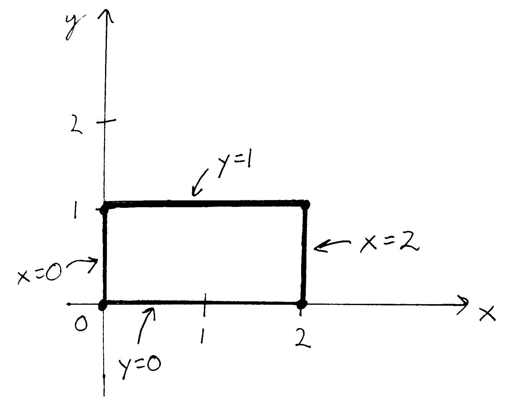
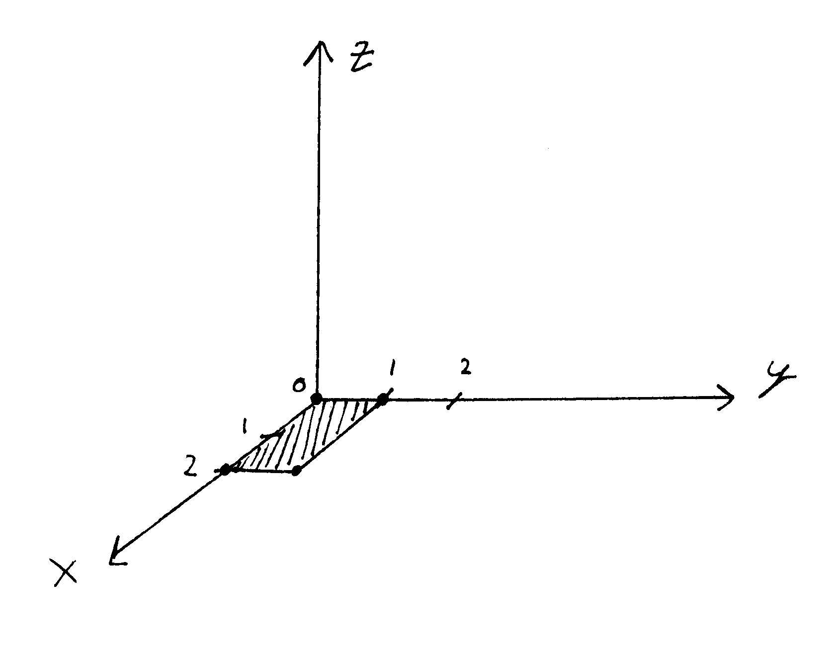
In multi-variable calculus, instead of endpoints on a closed interval, we now have boundaries (2-D curves) on a closed region. Once again, we're adding an extra dimension and going from points in a 2D plane to curves in 3D space. For our region, those boundaries are specified by the equations \(y = 0\), \(y = 1\), \(x = 0\), and \(x = 2\). We'll call those boundaries A, B, C, and D, respectively. The function \((x, y)\) is like a funny-shaped blanket laying over (or under) the x-y plane. The region we've drawn is like the shadow cast by the piece of that blanket we're interested in.

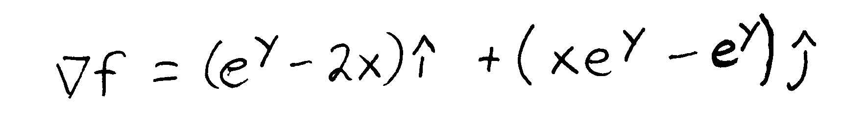
Ok, first step: we're going to take the gradient of our function (recall that it is \(f(x,y)=xe^y-x^2-e^y\)):

Setting the components equal to 0, we get a system of equations:

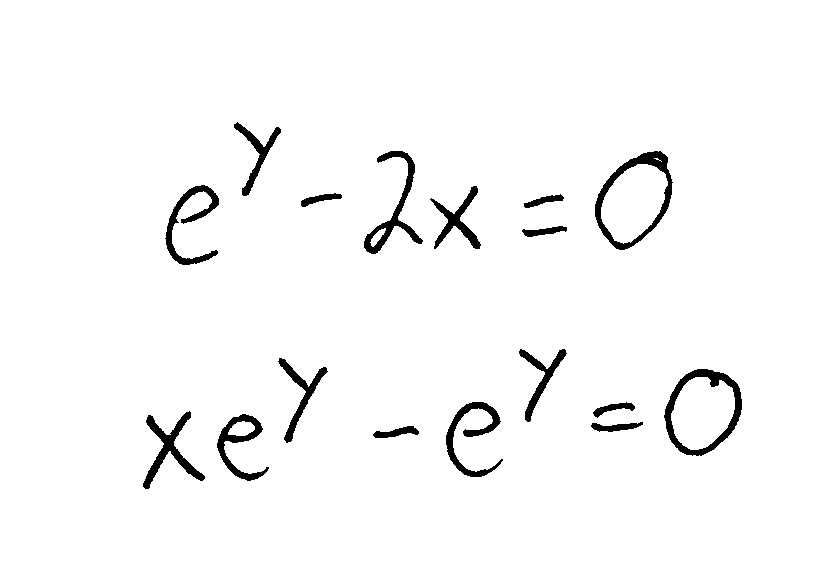
Solving this system, we get:

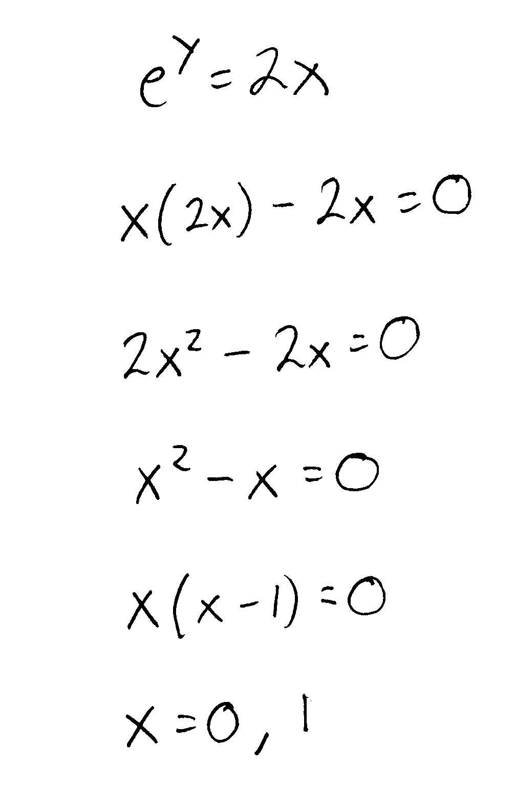
Plugging \(x = 0\) back into the system of equations, we get:

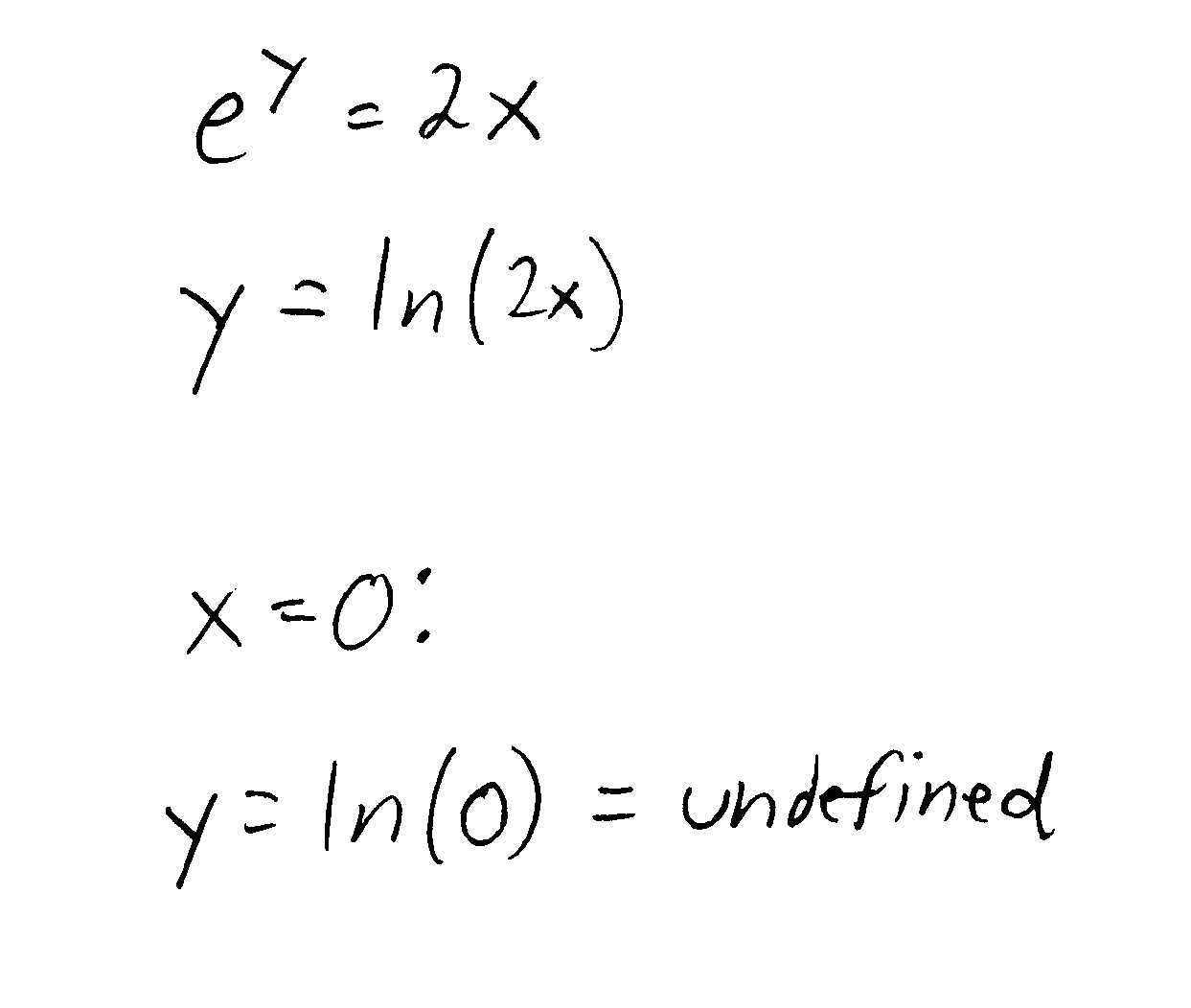
\(y\) is undefined at this point (it goes off to \(-\infty\)), so we ignore it. For \(x = 1\) we get:

Since we are only concerned with points inside our region, we must check to make sure this point does indeed lie inside the region. It does.

The next step is to take a look at the boundaries. What does that mean? It means that we are going to substitute the equation of each boundary into \(f(x, y)\), giving us a function of a single variable. We'll call those boundary functions \(f_{A}\), \(f_{B}\), \(f_{C}\), and \(f_{D}\), corresponding to each of our boundaries.

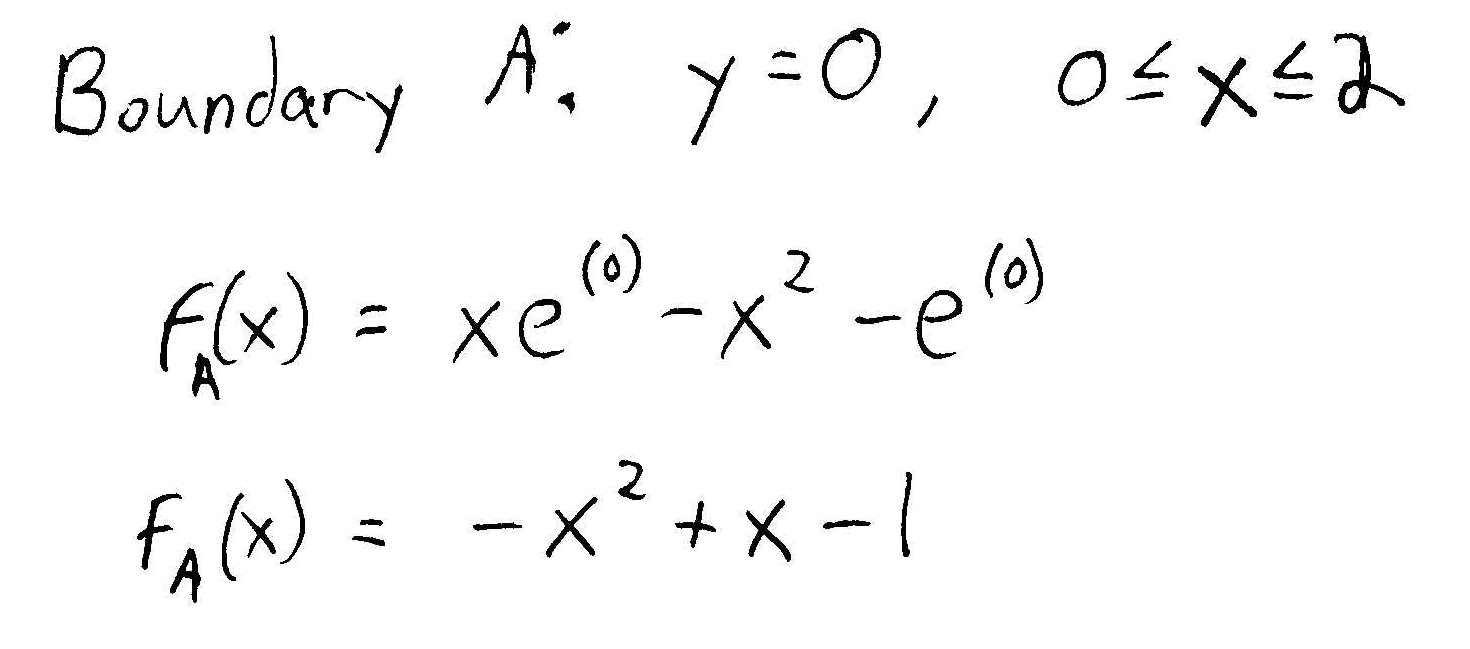
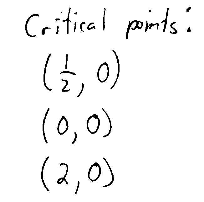
For boundary \(A\) (\(y = 0\)), we get:

Now, we're going to find the maximum and minimum values of this boundary function, which itself is bounded by two endpoints (\(x = 0\) and \(x = 2\)). Taking the derivative and setting it equal to zero, we get:

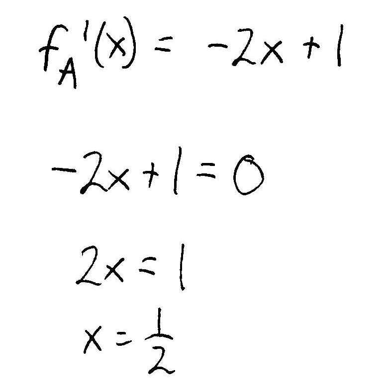
Since \(y = 0\) no matter where we are on the boundary, then together with the two endpoints we get 3 critical points:

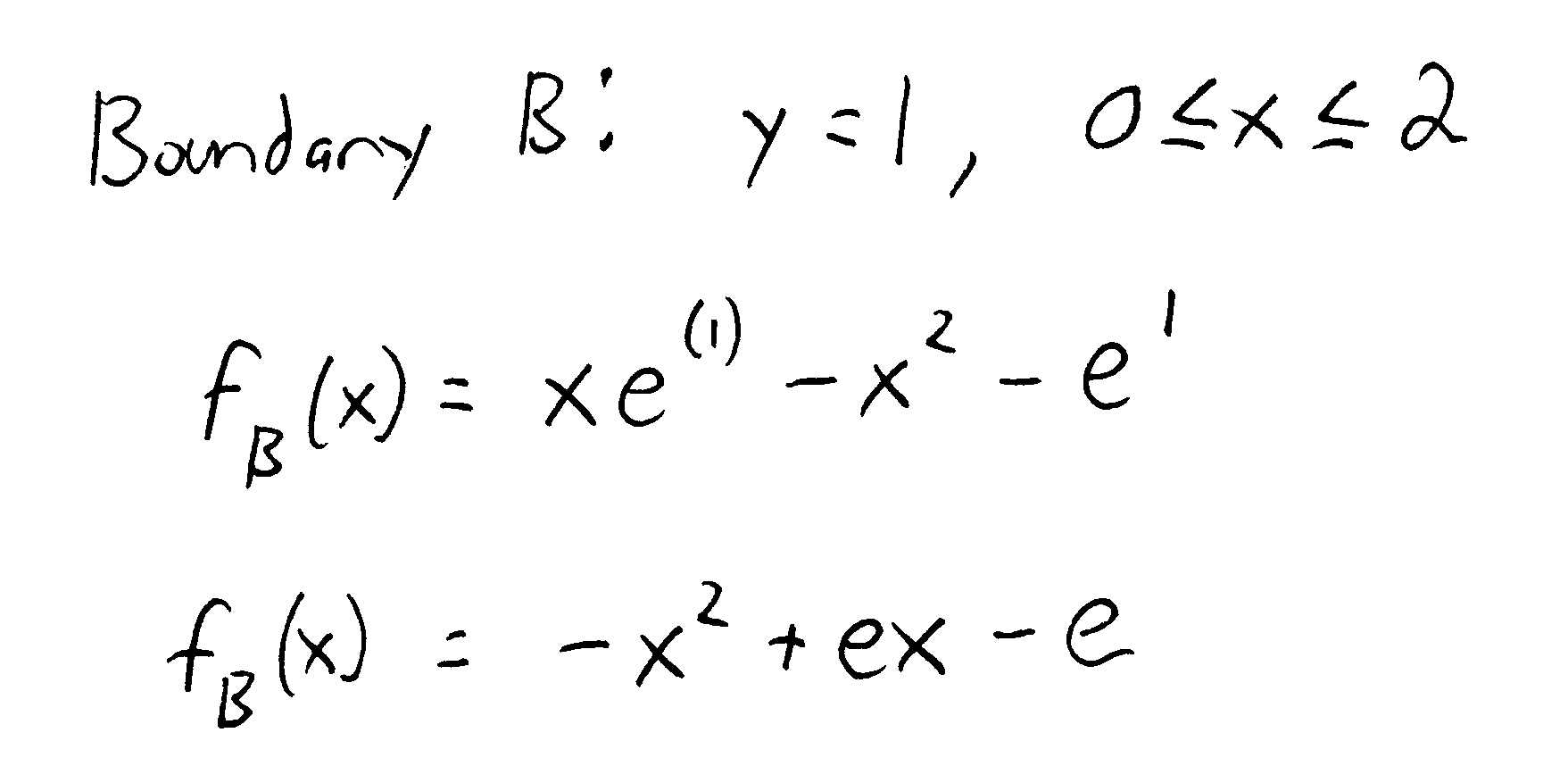
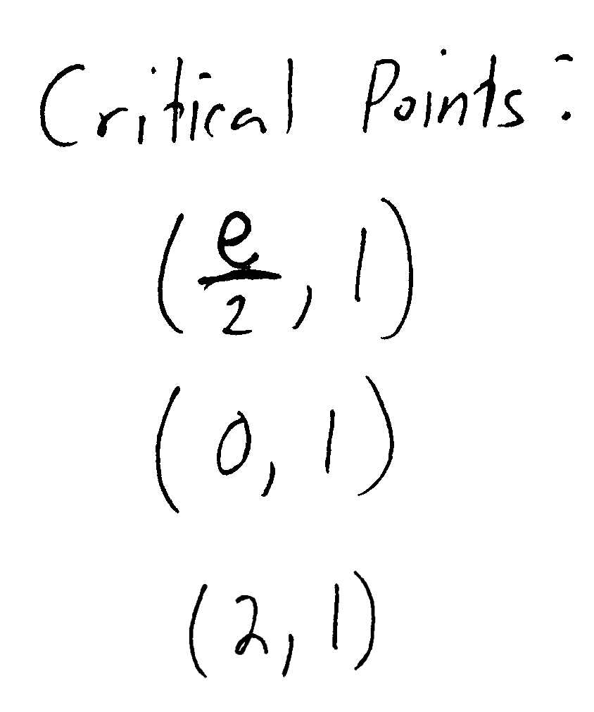
For boundary \(B\) (\(y = 1\)), we can do the same thing (remember to include the endpoints of boundary \(B\), too!):

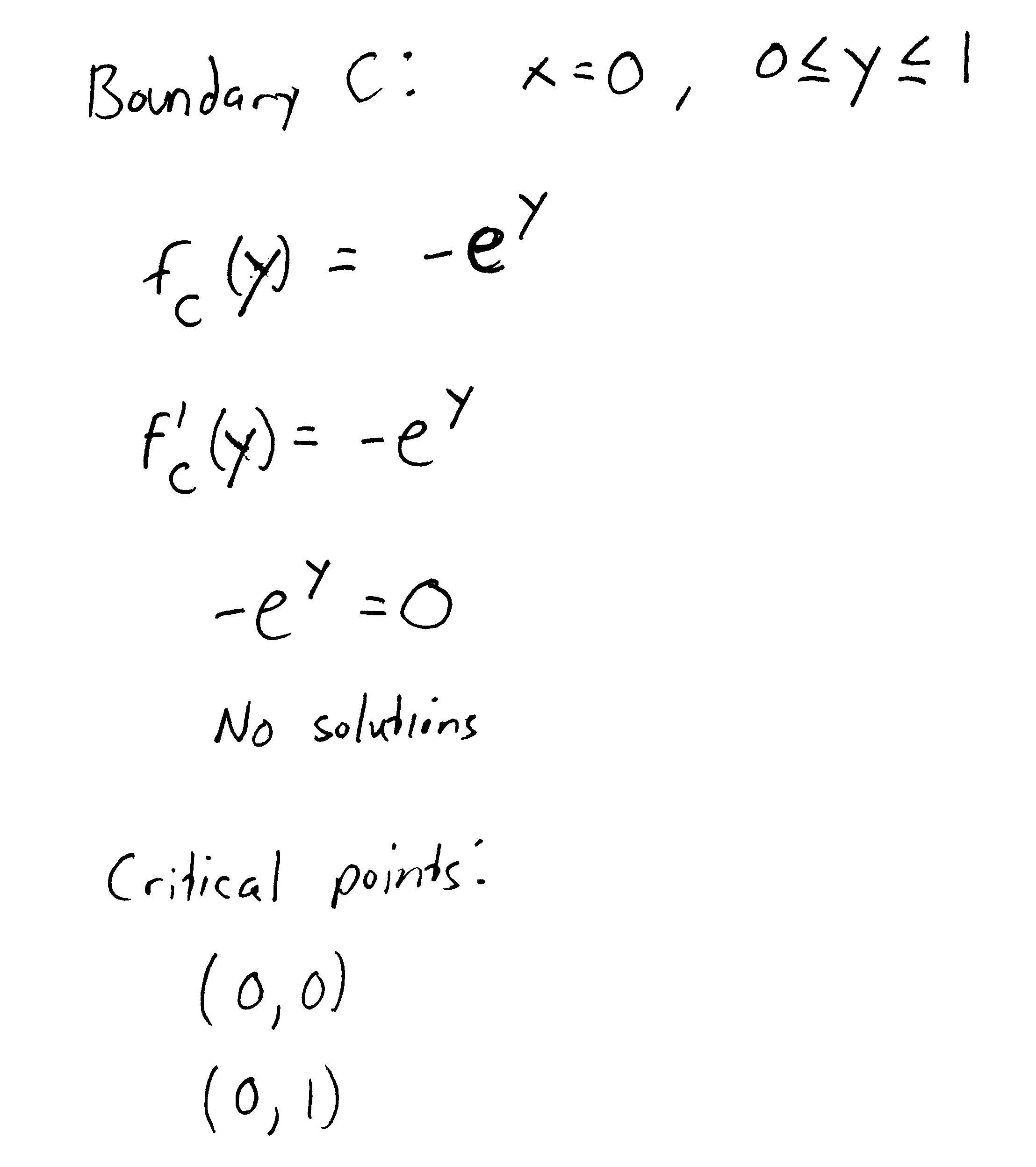
For boundary \(C\) (\(x = 0\)), we get:

And for boundary \(D\) (\(x = 2\)), we get:

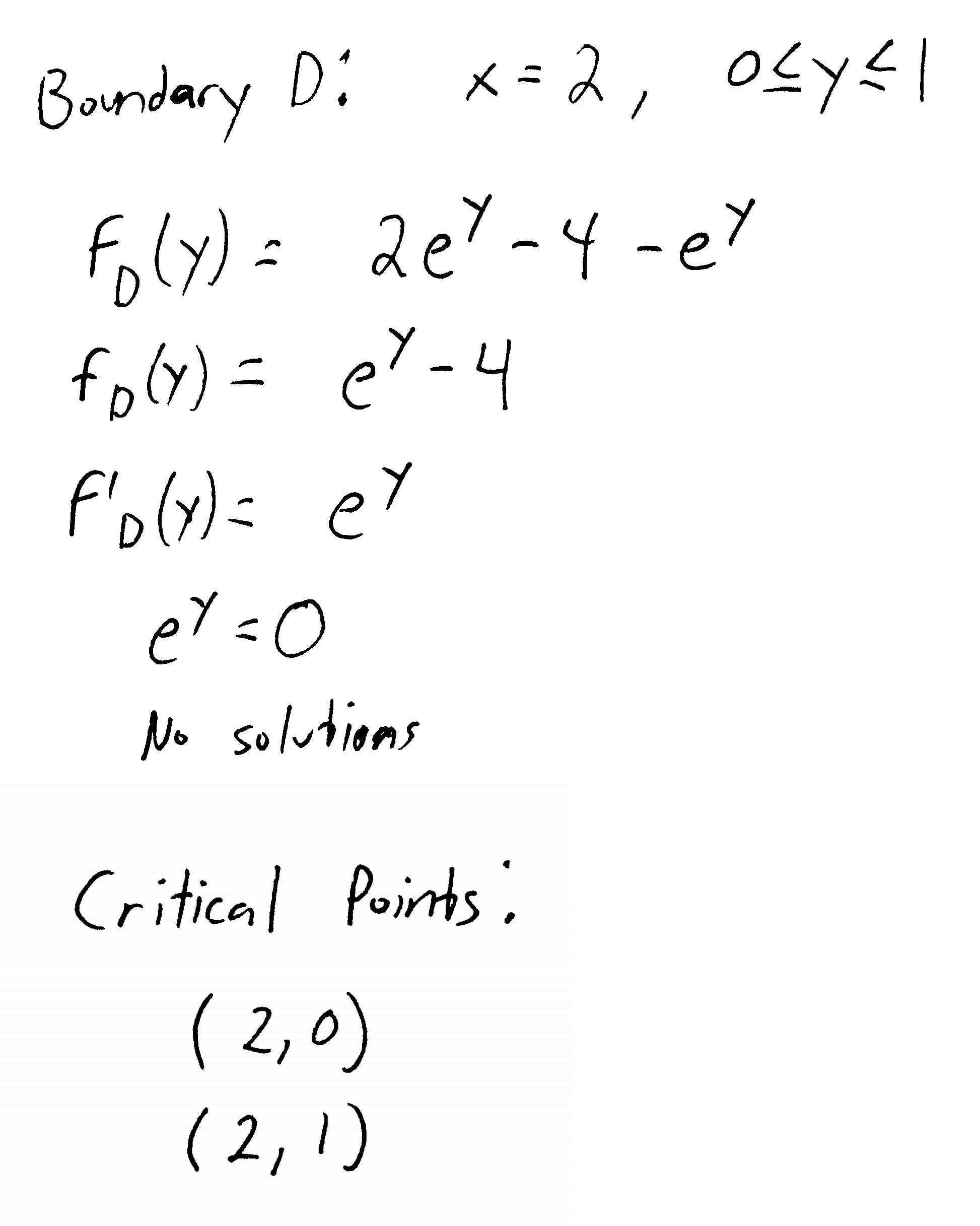
Compiling the critical points from the gradient of \(f(x, y)\) together with the points from each of the boundaries, we can make a nice neat table:

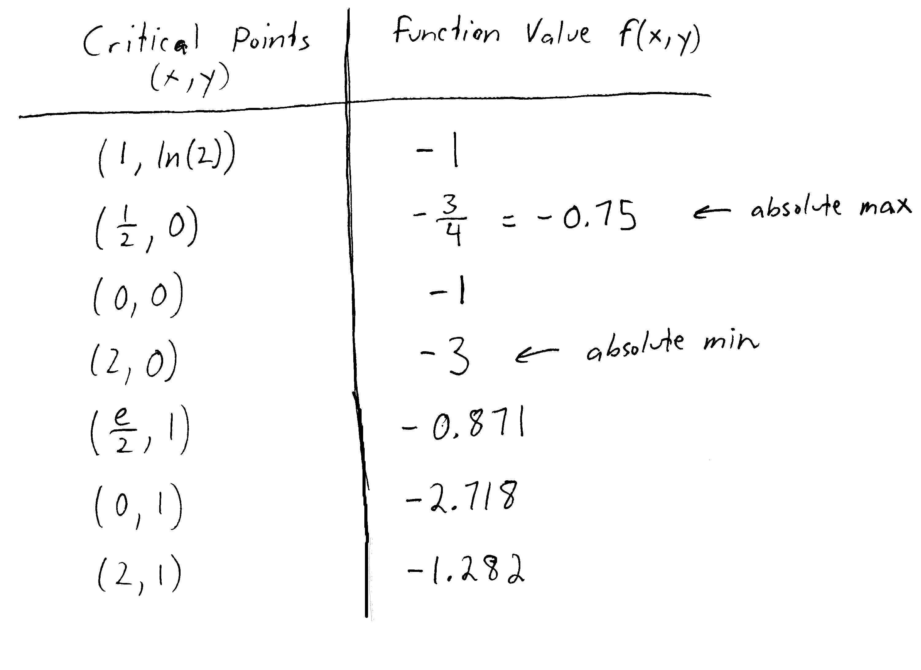
To find the absolute maximum and minimum, we simply evaluate \(f(x, y)\) at each of these points. The largest value is our maximum at \((\frac{1}{2},0)\), and the smallest value is our minimum at \((2,0)\). That's it! Unlike unbounded extreme value problems, there is no need to do a second derivative test. This is because we're not concerned with whether a particular point is a local minimum, maximum, or what have you. All we care about is whether a point has the absolute maximum or minimum value in our closed, bounded region.

If we look at the graph of this function in Mathematica, we can actually see the location of the maximum and minimum values of the function on the region:

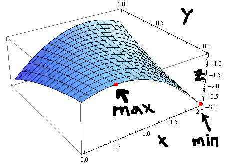
And there you have it. Extreme values. Extreme math.